Overfitting vs Underfitting: The Ultimate Guide to Mastering Perfect Model Balance
Have you ever built a machine learning model that worked brilliantly on your training data but crashed and burned when faced with real-world data? Or perhaps you’ve created a model so simple that it missed obvious patterns? If so, you’ve experienced the classic machine learning dilemma of overfitting vs underfitting.
As someone who’s spent years training models for both research and production, I can tell you that finding the right balance is both challenging and critical. In this guide, I’ll walk you through everything I’ve learned about identifying and fixing these common issues—with practical code examples you can apply to your own projects.
What You’ll Learn in This Guide
- What overfitting and underfitting really mean (in plain English!)
- How to visually spot these problems in your models
- Step-by-step code solutions you can implement today
- Real-world strategies I’ve used to find the perfect model complexity
- Expert tips for production-ready machine learning
What Is Overfitting vs Underfitting?
Let’s break down these concepts in simple terms—because understanding the problem is half the solution.
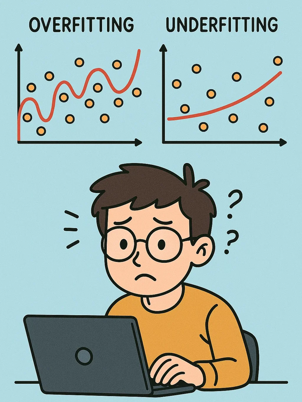
Overfitting: When Your Model Studies Too Hard
Imagine studying for an exam by memorizing all the answers to practice questions instead of understanding the underlying concepts. That’s essentially what happens when a model overfits.
An overfit model is like that student who memorizes the textbook but can’t solve new problems.
Signs you’re dealing with overfitting:
- Your model aces the training data (often with 95%+ accuracy)
- It performs poorly on validation or test data
- You see a large gap between training and validation metrics
- Your model has suspiciously high complexity for the problem at hand
Underfitting: When Your Model Doesn’t Study Enough
On the flip side, underfitting happens when your model is too simple to capture what’s really going on in your data.
An underfit model is like trying to understand quantum physics after reading only the first chapter of “Physics for Dummies.”
Signs of underfitting include:
- Poor performance on training data
- Similarly poor performance on validation/test data
- Little difference between training and validation metrics (but both are bad)
- The model makes overly simplistic predictions
Side-by-Side Comparison
| Aspect | Overfitting | Underfitting |
|---|---|---|
| Training Accuracy | High | Low |
| Test Accuracy | Low | Low |
| Model Complexity | Too complex | Too simple |
| Bias | Low | High |
| Variance | High | Low |
| Fix Strategies | Simplify, Regularize, Early stopping | Add complexity, Feature engineering |
The Bias-Variance Tradeoff Visualized
At the heart of this battle between overfitting and underfitting lies the bias-variance tradeoff—a fundamental concept in machine learning that’s worth understanding.
- High Bias (Underfitting): Your model makes strong assumptions about the data structure, missing important patterns
- High Variance (Overfitting): Your model is too sensitive to small fluctuations in the training data
- Balanced Model: Captures true underlying patterns without getting distracted by noise
Detecting Overfitting and Underfitting in Your Models
Let’s get practical with some code. I’ve found visualization to be incredibly helpful when diagnosing these issues.
import numpy as np
import matplotlib.pyplot as plt
from sklearn.model_selection import train_test_split
from sklearn.preprocessing import PolynomialFeatures
from sklearn.linear_model import LinearRegression
from sklearn.metrics import mean_squared_error
from sklearn.pipeline import make_pipeline

# Generate synthetic data with some noise
np.random.seed(42)
X = np.sort(np.random.rand(100, 1), axis=0)
y = np.sin(2 * np.pi * X).ravel() + np.random.normal(0, 0.1, X.shape[0])

# Split data into training and testing sets
X_train, X_test, y_train, y_test = train_test_split(X, y, test_size=0.3, random_state=42)

# Function to fit polynomial regression models of different degrees
def fit_polynomial_regression(degree):
    model = make_pipeline(PolynomialFeatures(degree), LinearRegression())
    model.fit(X_train, y_train)

    # Generate predictions for plotting
    X_plot = np.linspace(0, 1, 100).reshape(-1, 1)
    y_plot = model.predict(X_plot)

    # Calculate training and testing errors
    train_error = mean_squared_error(y_train, model.predict(X_train))
    test_error = mean_squared_error(y_test, model.predict(X_test))

    return X_plot, y_plot, train_error, test_error

# Models with different complexity levels
degrees = [1, 3, 15]
models = []

plt.figure(figsize=(16, 4))

for i, degree in enumerate(degrees):
    X_plot, y_plot, train_error, test_error = fit_polynomial_regression(degree)
    models.append((degree, X_plot, y_plot, train_error, test_error))

    # Create subplot
    plt.subplot(1, 3, i+1)
    plt.scatter(X_train, y_train, color='blue', alpha=0.5, label='Training data')
    plt.scatter(X_test, y_test, color='green', alpha=0.5, label='Testing data')
    plt.plot(X_plot, y_plot, color='red', label=f'Polynomial (degree={degree})')
    plt.ylim(-1.5, 1.5)
    plt.title(f'Degree {degree}\nTrain MSE: {train_error:.4f}, Test MSE: {test_error:.4f}')
    plt.legend()

plt.tight_layout()
plt.show()
This code demonstrates three key scenarios I often encounter:
- Underfitting (Degree 1): A linear model that’s too simple to capture the sinusoidal pattern
- Good Fit (Degree 3): A model with appropriate complexity that captures the true pattern
- Overfitting (Degree 15): A complex model that fits training data perfectly but fails on test data
It’s almost always helpful to visualize learning curves to see how errors change with model complexity:
# Plot learning curves
degrees = list(range(1, 20))
train_errors = []
test_errors = []

for degree in degrees:
    _, _, train_error, test_error = fit_polynomial_regression(degree)
    train_errors.append(train_error)
    test_errors.append(test_error)

plt.figure(figsize=(10, 6))
plt.plot(degrees, train_errors, 'o-', color='blue', label='Training error')
plt.plot(degrees, test_errors, 'o-', color='green', label='Testing error')
plt.xlabel('Polynomial Degree')
plt.ylabel('Mean Squared Error')
plt.title('Learning Curves: Error vs. Model Complexity')
plt.legend()
plt.grid(True)
plt.show()
7 Practical Strategies to Fix Overfitting
I’ve battled overfitting countless times. Here are the strategies that have consistently saved my models:
1. Collect More Data
In my experience, nothing beats having more training examples. More data helps models learn true patterns rather than noise. If collecting more data isn’t feasible, consider data augmentation techniques.
2. Feature Selection and Dimensionality Reduction
I’ve often found that removing unnecessary features can prevent models from learning noise:
from sklearn.feature_selection import SelectFromModel
from sklearn.ensemble import RandomForestRegressor

# Example of feature selection
selector = SelectFromModel(RandomForestRegressor(n_estimators=100, random_state=42))
selector.fit(X_train, y_train)

# Get selected features
X_train_selected = selector.transform(X_train)
X_test_selected = selector.transform(X_test)

print(f"Original features: {X_train.shape[1]}")
print(f"Selected features: {X_train_selected.shape[1]}")
3. Regularization: My Go-To Solution
Adding penalty terms to prevent large coefficients helps control model complexity:
from sklearn.linear_model import Ridge, Lasso

# Ridge Regression (L2 regularization)
ridge_model = Ridge(alpha=1.0)  # alpha controls regularization strength
ridge_model.fit(X_train, y_train)
ridge_train_score = ridge_model.score(X_train, y_train)
ridge_test_score = ridge_model.score(X_test, y_test)

# Lasso Regression (L1 regularization)
lasso_model = Lasso(alpha=0.1)
lasso_model.fit(X_train, y_train)
lasso_train_score = lasso_model.score(X_train, y_train)
lasso_test_score = lasso_model.score(X_test, y_test)

print(f"Ridge - Train R²: {ridge_train_score:.4f}, Test R²: {ridge_test_score:.4f}")
print(f"Lasso - Train R²: {lasso_train_score:.4f}, Test R²: {lasso_test_score:.4f}")
4. Early Stopping
This technique has saved me countless hours—stop training when validation metrics begin to worsen:
pythonfrom sklearn.ensemble import GradientBoostingRegressor
from sklearn.model_selection import train_test_split

# Split training data to create a validation set
X_train, X_val, y_train, y_val = train_test_split(
    X_train, y_train, test_size=0.2, random_state=42
)

# Train with early stopping
gb_model = GradientBoostingRegressor(
    n_estimators=1000,  # Maximum number of estimators
    learning_rate=0.1,
    subsample=0.8,
    random_state=42,
    validation_fraction=0.2,
    n_iter_no_change=10,  # Stop if no improvement after 10 iterations
    tol=1e-4
)

gb_model.fit(X_train, y_train)

# The model automatically used early stopping
print(f"Optimal number of estimators: {gb_model.n_estimators_}")
print(f"Best validation score: {gb_model.best_score_:.4f}")
5. Dropout and Batch Normalization for Neural Networks
For deep learning projects, I’ve found these techniques indispensable:
pythonimport tensorflow as tf
from tensorflow.keras.models import Sequential
from tensorflow.keras.layers import Dense, Dropout, BatchNormalization
from tensorflow.keras.callbacks import EarlyStopping

# Define model with dropout and batch normalization
model = Sequential([
    Dense(128, activation='relu', input_shape=(X_train.shape[1],)),
    BatchNormalization(),
    Dropout(0.3),  # Drop 30% of neurons during training
    Dense(64, activation='relu'),
    BatchNormalization(),
    Dropout(0.3),
    Dense(1)
])

# Compile model
model.compile(optimizer='adam', loss='mse')

# Early stopping callback
early_stopping = EarlyStopping(
    monitor='val_loss',
    patience=10,
    restore_best_weights=True
)

# Train with validation data
history = model.fit(
    X_train, y_train,
    validation_data=(X_val, y_val),
    epochs=200,
    callbacks=[early_stopping],
    batch_size=32,
    verbose=0
)
6. Cross-Validation
Cross-validation has consistently helped me assess model performance more reliably:
from sklearn.model_selection import cross_val_score
from sklearn.ensemble import RandomForestRegressor

# 5-fold cross-validation
model = RandomForestRegressor(n_estimators=100, random_state=42)
cv_scores = cross_val_score(model, X_train, y_train, cv=5, scoring='neg_mean_squared_error')

print(f"Cross-validation MSE: {-cv_scores.mean():.4f} ± {cv_scores.std():.4f}")
7. Ensemble Methods
Combining multiple models often gives me more robust predictions:
from sklearn.ensemble import VotingRegressor
from sklearn.linear_model import ElasticNet

# Create base models
models = [
    ('ridge', Ridge(alpha=1.0)),
    ('rf', RandomForestRegressor(n_estimators=100, max_depth=10)),
    ('elastic', ElasticNet(alpha=0.1, l1_ratio=0.5))
]

# Create ensemble
ensemble = VotingRegressor(estimators=models)
ensemble.fit(X_train, y_train)

# Evaluate
ensemble_train_score = ensemble.score(X_train, y_train)
ensemble_test_score = ensemble.score(X_test, y_test)

print(f"Ensemble - Train R²: {ensemble_train_score:.4f}, Test R²: {ensemble_test_score:.4f}")
5 Effective Ways to Combat Underfitting
When my models are too simple, here’s what I typically do:
1. Increase Model Complexity
Add more features or use more sophisticated models:
from sklearn.ensemble import RandomForestRegressor
from sklearn.svm import SVR

# Random Forest with more trees and depth
rf_model = RandomForestRegressor(
    n_estimators=100,
    max_depth=None,  # Allow full depth
    min_samples_split=2,
    random_state=42
)
rf_model.fit(X_train, y_train)
rf_train_score = rf_model.score(X_train, y_train)
rf_test_score = rf_model.score(X_test, y_test)

# Support Vector Machine with nonlinear kernel
svm_model = SVR(kernel='rbf', C=100, gamma='auto')
svm_model.fit(X_train, y_train)
svm_train_score = svm_model.score(X_train, y_train)
svm_test_score = svm_model.score(X_test, y_test)

print(f"Random Forest - Train R²: {rf_train_score:.4f}, Test R²: {rf_test_score:.4f}")
print(f"SVM - Train R²: {svm_train_score:.4f}, Test R²: {svm_test_score:.4f}")
2. Feature Engineering
This is where domain knowledge comes in handy—create new features that better capture the underlying patterns:
from sklearn.preprocessing import PolynomialFeatures

# Create polynomial features
poly = PolynomialFeatures(degree=3, include_bias=False)
X_train_poly = poly.fit_transform(X_train)
X_test_poly = poly.transform(X_test)

# Train linear model on polynomial features
linear_model = LinearRegression()
linear_model.fit(X_train_poly, y_train)
linear_train_score = linear_model.score(X_train_poly, y_train)
linear_test_score = linear_model.score(X_test_poly, y_test)

print(f"Polynomial Features - Train R²: {linear_train_score:.4f}, Test R²: {linear_test_score:.4f}")
3. Reduce Regularization
If your model is underfit, try reducing regularization strength:
# Ridge with lower regularization strength
ridge_weak = Ridge(alpha=0.01)  # Lower alpha means less regularization
ridge_weak.fit(X_train, y_train)
ridge_weak_train_score = ridge_weak.score(X_train, y_train)
ridge_weak_test_score = ridge_weak.score(X_test, y_test)

print(f"Weak Ridge - Train R²: {ridge_weak_train_score:.4f}, Test R²: {ridge_weak_test_score:.4f}")
4. Try More Powerful Models
Sometimes you need to step up to more sophisticated algorithms:
from xgboost import XGBRegressor
from lightgbm import LGBMRegressor

# XGBoost model
xgb_model = XGBRegressor(
    n_estimators=100,
    learning_rate=0.1,
    max_depth=7,
    random_state=42
)
xgb_model.fit(X_train, y_train)
xgb_train_score = xgb_model.score(X_train, y_train)
xgb_test_score = xgb_model.score(X_test, y_test)

# LightGBM model
lgb_model = LGBMRegressor(
    n_estimators=100,
    learning_rate=0.1,
    num_leaves=31,
    random_state=42
)
lgb_model.fit(X_train, y_train)
lgb_train_score = lgb_model.score(X_train, y_train)
lgb_test_score = lgb_model.score(X_test, y_test)

print(f"XGBoost - Train R²: {xgb_train_score:.4f}, Test R²: {xgb_test_score:.4f}")
print(f"LightGBM - Train R²: {lgb_train_score:.4f}, Test R²: {lgb_test_score:.4f}")
5. Increase Training Time
For neural networks and gradient boosting models, sometimes you just need more training epochs:
from sklearn.ensemble import GradientBoostingRegressor

# More iterations in gradient boosting
gb_model = GradientBoostingRegressor(
    n_estimators=500,  # More estimators
    learning_rate=0.05,  # Smaller learning rate
    random_state=42
)
gb_model.fit(X_train, y_train)
gb_train_score = gb_model.score(X_train, y_train)
gb_test_score = gb_model.score(X_test, y_test)

print(f"Gradient Boosting - Train R²: {gb_train_score:.4f}, Test R²: {gb_test_score:.4f}")
Finding the Sweet Spot: Cross-Validation in Action
Cross-validation is my secret weapon for finding the optimal model complexity. Here’s how to implement it:
from sklearn.model_selection import GridSearchCV

# Parameters to try
param_grid = {
    'polynomialfeatures__degree': [1, 2, 3, 4, 5],
    'ridge__alpha': [0.001, 0.01, 0.1, 1.0, 10.0, 100.0]
}

# Create pipeline
pipeline = make_pipeline(
    PolynomialFeatures(include_bias=False),
    Ridge()
)

# Grid search with cross-validation
grid_search = GridSearchCV(
    pipeline,
    param_grid,
    cv=5,  # 5-fold cross-validation
    scoring='neg_mean_squared_error',
    n_jobs=-1  # Use all available cores
)

grid_search.fit(X_train, y_train)

# Print best parameters
print(f"Best parameters: {grid_search.best_params_}")
print(f"Best cross-validation score: {-grid_search.best_score_:.4f}")

# Evaluate on test set
best_model = grid_search.best_estimator_
test_score = best_model.score(X_test, y_test)
print(f"Test R²: {test_score:.4f}")
Real-World Example: California Housing Dataset
Let’s apply these concepts to a real-world dataset:
from sklearn.datasets import fetch_california_housing
from sklearn.preprocessing import StandardScaler
from sklearn.model_selection import learning_curve

# Load California housing dataset
housing = fetch_california_housing()
X, y = housing.data, housing.target

# Scale features
scaler = StandardScaler()
X_scaled = scaler.fit_transform(X)

# Split data
X_train, X_test, y_train, y_test = train_test_split(
    X_scaled, y, test_size=0.2, random_state=42
)

# Compare different model complexities
models = {
    'Linear Regression (Underfitting)': LinearRegression(),
    'Random Forest (Good Fit)': RandomForestRegressor(n_estimators=100, max_depth=10, random_state=42),
    'Random Forest (Overfitting)': RandomForestRegressor(n_estimators=100, max_depth=None, min_samples_leaf=1, random_state=42)
}

for name, model in models.items():
    # Fit and evaluate model
    model.fit(X_train, y_train)
    train_score = model.score(X_train, y_train)
    test_score = model.score(X_test, y_test)
    print(f"{name} - Train R²: {train_score:.4f}, Test R²: {test_score:.4f}")
5 Practical Tips for Production-Ready Models
After years of deploying models to production, here are my top tips:
- Always Monitor the Gap: Keep a close eye on the difference between training and validation performance.
- Use Learning Curves: Plotting learning curves helps visualize whether your model is overfitting or underfitting.
- Implement K-Fold Cross-Validation: For smaller datasets, use k-fold cross-validation to get more reliable estimates of model performance.
- Consider Ensemble Methods: Techniques like stacking or blending often balance bias and variance effectively.
- Continuously Evaluate on New Data: Regularly monitor model performance to detect concept drift.
Frequently Asked Questions
What’s the most common cause of overfitting?
In my experience, the most common cause is having too few training examples relative to the model complexity. This is especially true with deep learning models that have millions of parameters but are trained on just thousands of examples.
How do I know if I should focus on fixing overfitting or underfitting?
Start by looking at your training metrics. If your model performs poorly even on training data, you’re likely underfitting. If it performs exceptionally well on training data but poorly on validation data, you’re likely overfitting.
Can a model both overfit and underfit at the same time?
Yes! Different parts of your model can exhibit different behaviors. For example, a neural network might overfit to some features while underfitting to others. This is where techniques like regularization and feature engineering become particularly important.
What’s the best regularization technique?
There’s no one-size-fits-all answer. L1 regularization (Lasso) tends to work well when you suspect many features are irrelevant. L2 regularization (Ridge) works better when most features contribute somewhat. In practice, I often use ElasticNet, which combines both approaches.
How much data do I need to avoid overfitting?
The rule of thumb is to have at least 10 times as many training examples as you have features or parameters. For complex models like deep neural networks, you might need 100x or even 1000x more examples than parameters to avoid overfitting.
What’s the relationship between model complexity and training time?
More complex models typically take longer to train. However, they might also require more regularization, which can increase training time further. It’s a balancing act—you want just enough complexity to capture the underlying patterns without unnecessary computational burden.
Should I always use cross-validation?
For small to medium-sized datasets, absolutely. However, for very large datasets, a simple train/validation/test split might be sufficient and more computationally efficient.
Conclusion: The Art and Science of Model Tuning
Finding the perfect balance between overfitting and underfitting is both an art and a science. It requires understanding your data, choosing appropriate models, and applying the right techniques to control model complexity.
By implementing the practical strategies outlined in this guide, you’ll be better equipped to build machine learning models that generalize well to new data—the ultimate goal of any production-ready solution.
Remember these key signs:
- Underfitting: Poor performance on both training and test data
- Overfitting: Excellent training performance but poor test performance
- Just Right: Good performance on both with a minimal gap
With these tools and techniques, you’re now ready to tackle the bias-variance tradeoff with confidence and build better machine learning models.
References
- Google Developers. (2022). Machine Learning: Generalization. Google Machine Learning Crash Course.
- Brownlee, J. (2023). How to Control Model Complexity. Machine Learning Mastery.
- AWS. (2024). Preventing Overfitting in Machine Learning Models. Amazon Web Services Machine Learning Blog.
- Scikit-learn. (2024). Model Selection: Underfitting vs. Overfitting. Scikit-learn Documentation.
- DeepAI. (2024). Bias-Variance Tradeoff. DeepAI.
- TensorFlow. (2024). Regularization for Simplicity. TensorFlow Tutorials.
- Stanford CS229. (2023). Bias-Variance and Error Analysis. Stanford University Machine Learning Course.
- Kaggle. (2024). Feature Engineering Techniques. Kaggle Learn.
- Microsoft. (2024). Model Validation in Azure Machine Learning. Microsoft Azure Documentation.
- PyTorch. (2024). Early Stopping to Avoid Overfitting. PyTorch Tutorials.